BCW2011 Refinancing Walkthrough#
Work through this page after BCW2011 Liquidation Walkthrough.
The code discussed here is:
src/example/BCW2011Refinancing.py
What To Watch#
By the end of this page, you should understand:
why Case II turns the left boundary into a financing problem,
why the solver must search both
v_leftands_max,how the issuance target
mis recovered numerically,how the
phi=1%andphi=0comparison maps to Figure 3.
Reproduction#
Run this example from the repository root:
MPLBACKEND=Agg uv run python src/example/BCW2011Refinancing.py
What Changes Relative To Liquidation#
The internal-financing region is unchanged. The state variable is still the cash-capital ratio w, and the interior HJB is still BCW Eq. (13). What changes is the lower boundary.
In liquidation, the lower boundary is exogenous:
In refinancing, the lower boundary becomes endogenous because the firm issues equity when it reaches zero cash instead of liquidating.
That change introduces:
a value-matching equation at the issuance point,
an optimal issuance-size condition at the post-issuance cash target
m.
Paper Equations Used In This Case#
Interior HJB And Investment Rule#
The interior still uses BCW Eq. (13) and Eq. (14):
Issuance Value Matching: Eq. (19)#
This says the value just before issuance equals the post-issuance firm value minus fixed and proportional issuance costs.
Optimal Issuance Size: Eq. (20)#
This is the smooth-pasting condition at the return cash-capital ratio m.
Right Boundary#
The right side is still pinned by BCW Eq. (16) and Eq. (17):
Why There Are Two Boundary Targets#
This case has two endogenous unknowns:
the payout boundary
\bar w,the left boundary value
p(0).
The issuance target m is not directly searched as a boundary variable. Instead, it is recovered from the solved grid as the point where:
This gives the repository workflow:
guess
v_left = p(0)ands_max = \bar w,solve the HJB on
[0, \bar w],read
moff the solved grid using the derivative condition,evaluate the issuance value-matching residual,
update both unknowns until the left issuance condition and right super-contact condition both hold.
That is why the script uses a two-target boundary search with method="hybr" instead of bisection.
How Those Equations Become FinHJB Objects#
Economic object |
FinHJB object |
Repository role |
|---|---|---|
benchmark parameters plus issuance costs |
|
stores |
boundary values |
|
exposes |
investment control |
|
stores |
Eq. (14) |
|
implicit update for |
Eq. (13) |
|
interior HJB |
Eq. (19) |
|
left-boundary target |
Eq. (20) |
|
recovers |
The important FinHJB design point is that m is not a separate state variable or separate boundary object. It is an economically meaningful interior point inferred from the solved grid.
Why hybr Is The Right Search Method Here#
The script searches two nonlinear targets simultaneously:
super_contact_residual(grid)for the payout boundary,refinancing_boundary_residual(grid)for the issuance boundary.
This is qualitatively different from liquidation:
liquidation has one scalar target and a robust bracket,
refinancing has a coupled system because moving
v_leftchanges the whole value function and therefore changes bothmand the right boundary geometry.
That is why the repository standardizes this case on hybr.
Figure 3: What The Comparison Means#
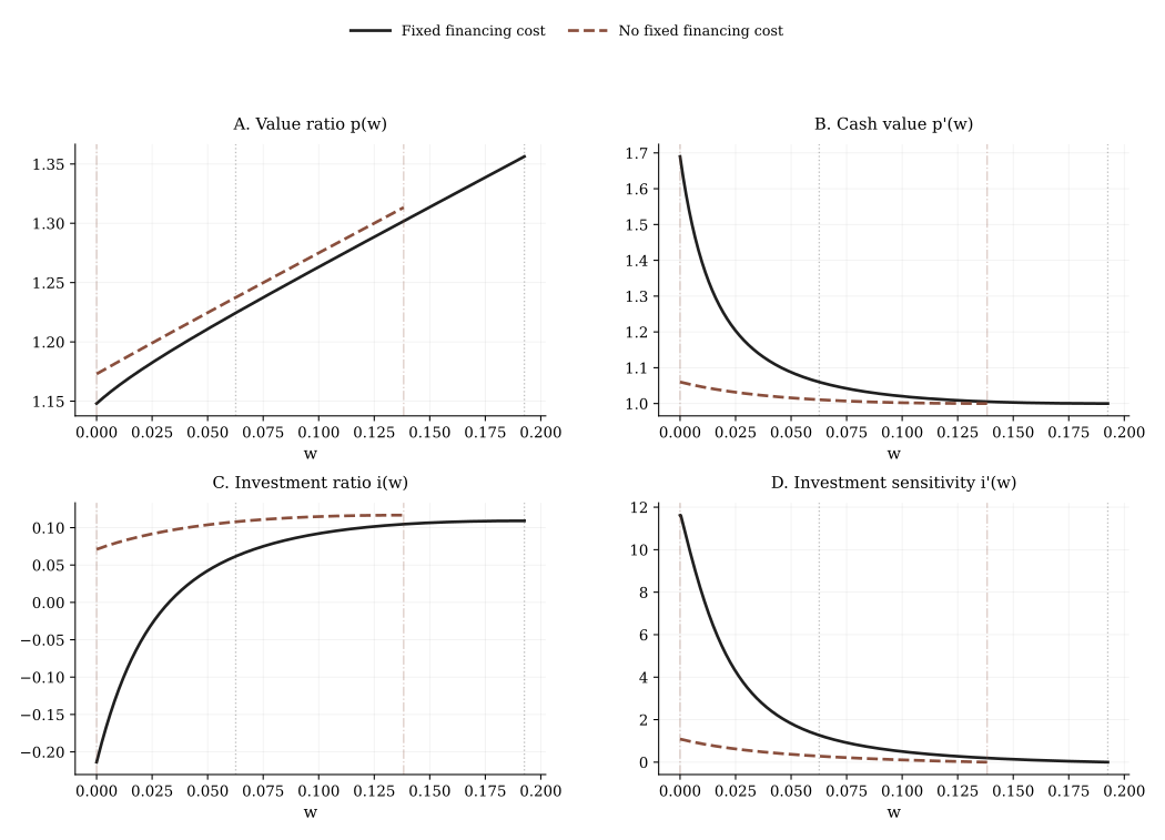
Panel A: p(w)#
The key comparison is at the left endpoint:
with costly issuance,
p(0)is still above liquidation value,with zero fixed issuance cost, the curve lifts further and the financing friction is milder.
This is the numerical version of BCW’s condition that refinancing is globally preferred when p(0) > l.
Panel B: p'(w)#
Fixed issuance costs increase the marginal value of cash in low-cash states because internal liquidity helps the firm avoid paying those fixed costs too often.
Panel C: i(w)#
Investment is less distorted than in liquidation, but still below first best when financing is costly.
Panel D: i'(w)#
The steepness of i'(w) near the left side is a compact way to see how financing frictions transmit into real decisions.
Stable Quantitative Targets#
Healthy runs usually show:
with
phi=1%:\bar w \approx 0.19,m \approx 0.06,p(0) > l,with
phi=0:\bar w \approx 0.14,m \approx 0,p'(m) \approx 1.06in both scenarios.
These are exactly the targets to compare against Figure 3.
Code Inspection Pattern#
from src.example.BCW2011Refinancing import run_case

bundle = run_case(number=1000)
for label, result in bundle["results"].items():
    print(label, result["summary"])
For this case, the most informative summary fields are:
return_cash_ratio,dv_at_m,p0_above_l,payout_boundary.
How To Adapt This Pattern#
Start from this case if your own model needs:
issuance instead of liquidation,
a left-boundary value-matching condition,
an interior target like
mdefined by a derivative condition,more than one searched boundary unknown.
This is the right template for many financing models even when the later hedging and credit-line extensions are unnecessary.