BCW2011 Hedging Walkthrough#
Work through this page after BCW2011 Refinancing Walkthrough.
The code discussed here is:
src/example/BCW2011Hedging.py
What To Watch#
By the end of this page, you should understand:
how BCW’s hedging case modifies the HJB rather than just adding a plotted series,
how Eq. (28)-(30) become a two-control FinHJB problem,
why the hedge rule splits into maximum-hedging, interior, and zero-hedging regions,
how the costly-margin solution differs from the frictionless comparison object.
Reproduction#
Run this example from the repository root:
MPLBACKEND=Agg uv run python src/example/BCW2011Hedging.py
What Changes Relative To Refinancing#
The hedging case keeps the same reduced state variable w = W/K, and it keeps the same issuance and payout logic as the refinancing case. The structural change is that the firm now chooses both:
investment
i(w),hedge demand
\psi(w).
This means the value function still solves on one state dimension, but the policy problem is now genuinely multi-control.
Paper Equations Used In This Case#
Costly-Margin HJB: Eq. (28)#
BCW’s HJB becomes:
After homogeneity reduction, the repository solves the one-dimensional form in w.
Margin Constraint: Eq. (29)#
With \rho > 0, BCW focuses on short futures positions, so \psi \leq 0.
Interior Hedge Rule: Eq. (30)#
This is the unconstrained interior hedge policy. The actual hedge rule is then clipped into the admissible regions:
\psi=-\piin the maximum-hedging region,Eq. (30) in the interior region,
\psi=0in the zero-hedging region.
Frictionless Comparison: Eq. (27)#
The paper’s no-margin benchmark fully eliminates systematic risk. In implementation, the repository does not solve a separate closed-form benchmark object outside FinHJB. Instead, it solves a comparison HJB with:
epsilon = 0,very large
pi,the same issuance/payout workflow,
the same plotting interface as the costly-margin case.
This gives a directly comparable numerical object for Figure 6.
How The Two-Control Problem Becomes FinHJB Code#
Economic object |
FinHJB object |
Repository role |
|---|---|---|
hedging parameters |
|
adds |
controls |
|
stores |
policy update |
|
computes both controls explicitly from the current grid |
HJB residual |
|
implements Eq. (28) in reduced form |
issuance and payout boundaries |
|
reused from the refinancing logic |
The design choice here is different from the single-control cases:
investmentandpsiare updated together in one explicit policy step,psi_interioris stored separately so the code can diagnosew_-andw_+even though the actual hedge rule is clipped.
Why The Solver Still Uses boundary_search()#
Even though the policy problem is richer, the state dimension is still one. The outer numerical problem still asks for:
the left issuance value,
the right payout boundary.
So the workflow stays:
solve the interior HJB for the current boundary guesses,
recover issuance information from
p'(w),update the boundary targets,
stop when issuance matching and payout super-contact both hold.
The script uses method="hybr" because these targets are coupled and the hedge control changes the curvature of the value function in a materially nonlinear way.
The Three Hedge Regions#
The repository extracts BCW’s two endogenous cutoffs from psi_interior:
w_-solves\psi^*(w_-) = -\pi,w_+solves\psi^*(w_+) = 0.
That gives the three-region interpretation:
w \leq w_-: maximum hedging,\psi=-\pi,w_- < w < w_+: interior hedging,\psi=\psi^*(w),w \geq w_+: no hedging,\psi=0.
This is one of the cleanest examples in the repository of using an auxiliary policy series both for plotting and for economic diagnostics.
Figure 6: How To Read The Comparison#
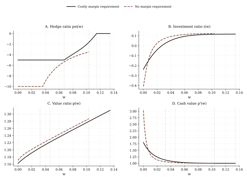
Panel A: \psi(w)#
The costly-margin solution shows BCW’s three regions. The frictionless comparison is clipped for display, matching the paper’s plotting convention.
Panel B: i(w)#
Hedging affects investment because better risk management changes both firm value and the marginal value of cash.
Panel C: p(w)#
The value-capital ratio is higher with better risk management, but the gain is strongest away from the most constrained states.
Panel D: p'(w)#
The marginal value of cash generally falls when the firm can hedge more effectively, except in the severe-constraint region where hedging capacity itself becomes liquidity-sensitive.
Stable Quantitative Targets#
Healthy runs usually show:
costly margin:
w_- \approx 0.07,w_+ \approx 0.11,\bar w \approx 0.14,\psi \in [-5, 0],frictionless comparison: payout occurs earlier than under costly margin,
the frictionless display line is clipped at
-10for the figure.
These are the right economic checks before you compare cosmetic line shapes.
Code Inspection Pattern#
from src.example.BCW2011Hedging import run_case

bundle = run_case(number=1000)
for label, result in bundle["results"].items():
    print(label, result["summary"])
The most informative outputs are:
psi,psi_interior,max_hedging_boundary,zero_hedging_boundary,return_cash_ratio.
How To Adapt This Pattern#
Start from this case if your own model has:
more than one control,
a control-dependent diffusion term,
an economically meaningful clipped interior control,
boundary logic that still looks like refinancing.
It is the right template for one-dimensional models whose complexity comes from policies, not from extra state variables.